Difference between revisions of "GW150914 VisIt Tutorial"
Bentivegna (talk | contribs) |
|||
| (25 intermediate revisions by 5 users not shown) | |||
| Line 1: | Line 1: | ||
| − | =Visualizing the spacetime with VisIt= | + | =Visualizing the spacetime of GW150914 with VisIt= |
| + | <!-- This page is not an orphan, it is linked to from the ET gallery example on BBH: https://einsteintoolkit.org/gallery/bbh/index.html --> | ||
==Installing VisIt== | ==Installing VisIt== | ||
| − | The 3D data output by the simulation (such as the metric, the extrinsic curvature, the curvature, and the apparent horizons) can be visualised with the | + | The 3D data output by the simulation (such as the metric, the extrinsic curvature, the curvature, and the apparent horizons) can be visualised with the <tt>VisIt</tt> package. <tt>VisIt</tt> can be obtained at the [https://visit-dav.github.io/visit-website/releases-as-tables/#latest VisIt download page]. |
| − | The simplest way to install VisIt is to download the ready-made executable for the right architecture (Linux, Mac OS X, and Windows are available). On Linux, this will download a tarball containing a directory | + | The simplest way to install <tt>VisIt</tt> is to download the ready-made executable for the right architecture (Linux, Mac OS X, and Windows are available). On Linux, this will download a tarball containing a directory |
visit<version number>.<architecture> | visit<version number>.<architecture> | ||
| Line 15: | Line 16: | ||
will launch the software. | will launch the software. | ||
| − | On Mac OS X, a .dmg file will be downloaded first, containing the | + | On Mac OS X, a .dmg file will be downloaded first, containing the <tt>VisIt.app</tt> executable. |
==Opening the databases== | ==Opening the databases== | ||
| − | Once the software is running, the button | + | Once the software is running, the button <tt>Open</tt> can be used to open files from the simulation. If you did not run the simulation yourself, you can obtain a copy of the output data sufficient for this tutorial from [http://dx.doi.org/10.5281/zenodo.155394 Zenodo]. |
| − | + | Make sure to select Open file as type: CarpetHDF5, otherwise VisIt may try to load the data using another format, and may crash. | |
| − | + | [[Image:vt-1.png]] | |
| − | + | If you are using the Simulation Factory to launch and manage the run, the data will be output under the directory <tt><basedir>/<simulation name>/output-<nnnn>/<parfile name></tt>, where <tt><nnnn></tt> is the number of the restart. There are essentially two types of files that can be visualised with VisIt: | |
| − | + | ||
| + | * Files from the thorn <tt>CarpetIOHDF5</tt>, with .h5 extension, which will be read by the CarpetHDF5 plugin in VisIt and represent the 1D, 2D, or 3D configuration of a specific field, on a number of constant-time spaces; | ||
| + | * Files from the thorn <tt>QuasiLocalMeasures</tt>, with .vtk extension, which are read natively by <tt>VisIt</tt> and represent the shape and properties of relevant 2D topological spheres, such as the apparent horizons, also at different times; | ||
==A visualization example== | ==A visualization example== | ||
| − | Let us, for instance, plot the configuration of the conformal factor | + | Let us, for instance, plot the configuration of the conformal factor <tt>ML_BSSN::phi</tt> on the xy plane, and superimpose the apparent horizon shapes. We first need to load the data for the conformal factor on this plane, using the Open button and selecting the correct path for the database <tt>phi.*.xy.h5</tt>. We can then generate the plot by clicking <tt>Add > Pseudocolor > ML_BSSN--phi</tt>. If the <tt>Auto Apply</tt> feature in <tt>VisIt</tt> is not selected, we need to click on <tt>Draw</tt> to make the plot appear. |
| − | [[Image: | + | [[Image:Openfiles.png]] |
| − | [[Image: | + | [[Image:vt-3.png]] |
| − | [[Image: | + | [[Image:vt-4.png]] |
| − | If necessary, we can tune the colormap until the plot looks like the one below (this result has been obtained by selecting the | + | If necessary, we can tune the colormap until the plot looks like the one below (this result has been obtained by selecting the <tt>Plot Attributes > Pseudocolor...</tt> menu and choosing a <tt>Skew</tt> value of 1000): |
| − | [[Image: | + | [[Image:vt-5.png]] |
| − | Next, we can plot the horizon surface of the first black hole by opening the | + | Next, we can plot the horizon surface of the first black hole by opening the <tt>surface01_*.vtk</tt> database, and using <tt>Add > Mesh > mesh</tt>. We can similarly add the second horizon by following the previous steps for the <tt>surface02_*.vtk</tt> database. |
| − | [[Image: | + | [[Image:vt-6.png]] |
| − | [[Image: | + | [[Image:vt-7.png]] |
| − | [[Image: | + | [[Image:vt-8.png]] |
| − | The plot depicts now the system’s conformal factor and horizons at t=0. To cycle through subsequent times, we need to create a database correlation first, telling | + | The plot depicts now the system’s conformal factor and horizons at t=0. To cycle through subsequent times, we need to create a database correlation first, telling <tt>VisIt</tt> how to match the time indices in the <tt>phi.*.xy.h5</tt>, <tt>surface01_*.vtk</tt>, and <tt>surface02_*.vtk</tt>. To create the database, we need to use the menu <tt>Controls > Database correlations</tt>, select <tt>New…</tt>, select the three databases on the left window (<tt>Sources</tt>) and move them right using the right arrow. Once the databases appear in the <tt>Correlated sources</tt> window, we can name the correlation, select <tt>Cycle</tt> for the correlation method, and click <tt>Create database correlation</tt>. Once the correlation is created, an <tt>Active time slider</tt> menu will appear just below the <tt>Active Source</tt> menu, indicating that our correlation is now controlling the slider; moving this slider will then step through the three databases simultaneously, making sure that all the plotted data refers to the same time coordinate. |
| − | + | <tt>VisIt</tt> provides a number of tools and options to tune this visualization, output it to image or movie files, save and restore sessions, remote visualization, and so on. More information can be found on the [https://wci.llnl.gov/simulation/computer-codes/visit/manuals Manuals page]. | |
| − | [[Image: | + | [[Image:vt-9.png]] [[Image:vt-10.png]] [[Image:vt-11.png]] |
Latest revision as of 17:52, 14 September 2022
Contents
Visualizing the spacetime of GW150914 with VisIt
Installing VisIt
The 3D data output by the simulation (such as the metric, the extrinsic curvature, the curvature, and the apparent horizons) can be visualised with the VisIt package. VisIt can be obtained at the VisIt download page.
The simplest way to install VisIt is to download the ready-made executable for the right architecture (Linux, Mac OS X, and Windows are available). On Linux, this will download a tarball containing a directory
visit<version number>.<architecture>
Changing to this directory, the command
bin/visit
will launch the software.
On Mac OS X, a .dmg file will be downloaded first, containing the VisIt.app executable.
Opening the databases
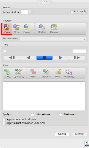
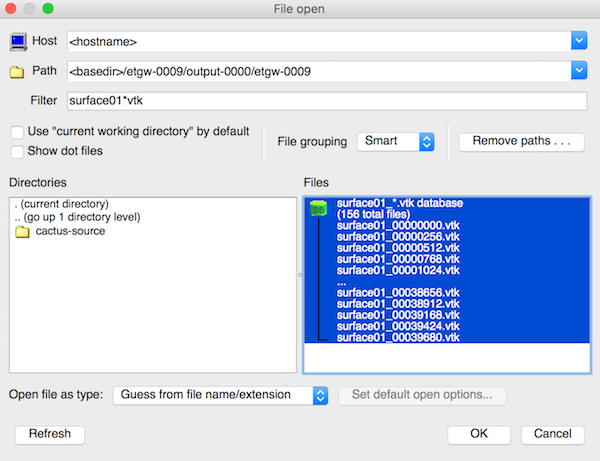
Once the software is running, the button Open can be used to open files from the simulation. If you did not run the simulation yourself, you can obtain a copy of the output data sufficient for this tutorial from Zenodo.
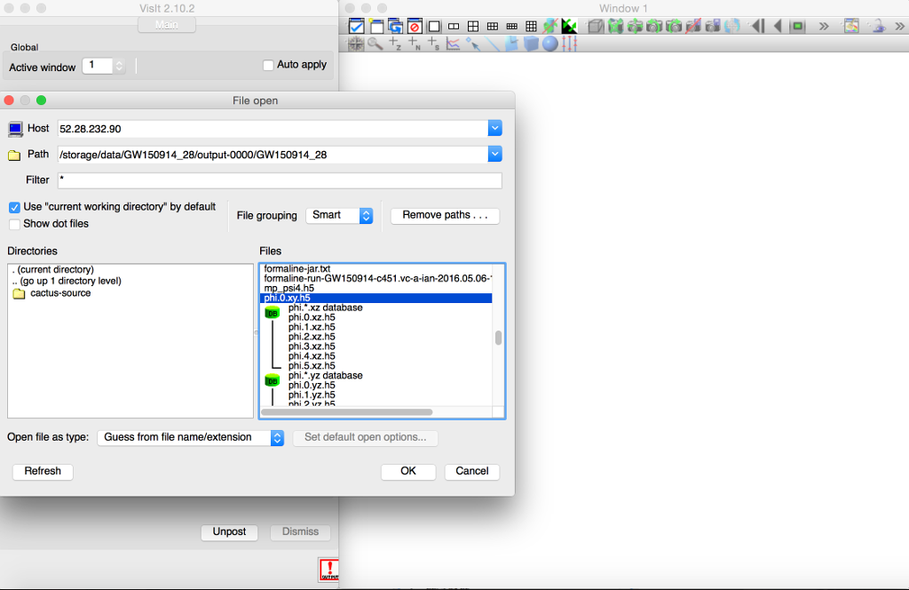
Make sure to select Open file as type: CarpetHDF5, otherwise VisIt may try to load the data using another format, and may crash.
If you are using the Simulation Factory to launch and manage the run, the data will be output under the directory <basedir>/<simulation name>/output-<nnnn>/<parfile name>, where <nnnn> is the number of the restart. There are essentially two types of files that can be visualised with VisIt:
- Files from the thorn CarpetIOHDF5, with .h5 extension, which will be read by the CarpetHDF5 plugin in VisIt and represent the 1D, 2D, or 3D configuration of a specific field, on a number of constant-time spaces;
- Files from the thorn QuasiLocalMeasures, with .vtk extension, which are read natively by VisIt and represent the shape and properties of relevant 2D topological spheres, such as the apparent horizons, also at different times;
A visualization example
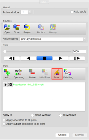
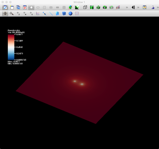
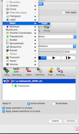
Let us, for instance, plot the configuration of the conformal factor ML_BSSN::phi on the xy plane, and superimpose the apparent horizon shapes. We first need to load the data for the conformal factor on this plane, using the Open button and selecting the correct path for the database phi.*.xy.h5. We can then generate the plot by clicking Add > Pseudocolor > ML_BSSN--phi. If the Auto Apply feature in VisIt is not selected, we need to click on Draw to make the plot appear.
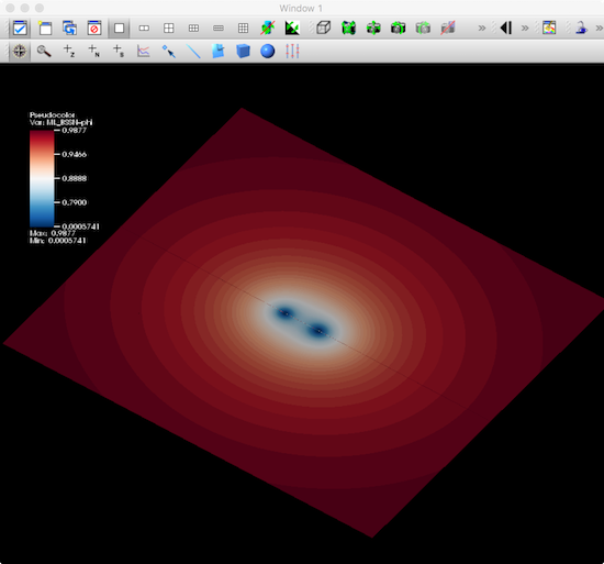
If necessary, we can tune the colormap until the plot looks like the one below (this result has been obtained by selecting the Plot Attributes > Pseudocolor... menu and choosing a Skew value of 1000):
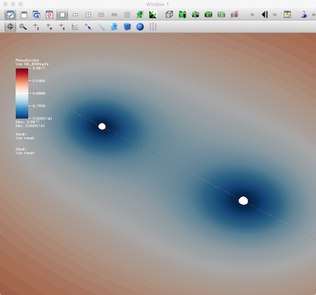
Next, we can plot the horizon surface of the first black hole by opening the surface01_*.vtk database, and using Add > Mesh > mesh. We can similarly add the second horizon by following the previous steps for the surface02_*.vtk database.
The plot depicts now the system’s conformal factor and horizons at t=0. To cycle through subsequent times, we need to create a database correlation first, telling VisIt how to match the time indices in the phi.*.xy.h5, surface01_*.vtk, and surface02_*.vtk. To create the database, we need to use the menu Controls > Database correlations, select New…, select the three databases on the left window (Sources) and move them right using the right arrow. Once the databases appear in the Correlated sources window, we can name the correlation, select Cycle for the correlation method, and click Create database correlation. Once the correlation is created, an Active time slider menu will appear just below the Active Source menu, indicating that our correlation is now controlling the slider; moving this slider will then step through the three databases simultaneously, making sure that all the plotted data refers to the same time coordinate.
VisIt provides a number of tools and options to tune this visualization, output it to image or movie files, save and restore sessions, remote visualization, and so on. More information can be found on the Manuals page.
