Tutorial for New Users
This section provides a simple guide for compiling and running an example parameter file for the Einstein Toolkit.
One complexity of high performance computing is the heterogeneous environments presented by different resources with different core software installations and local setups. For example, Einstein Toolkit codes require compiling with MPI and then running the resulting application in a batch queue. This complexity is hidden as much as possible in Cactus and accompanying tools such as the Simulation Factory.
The example worked through below assumes that you are using the NSF TeraGrid resource Queen Bee. If you don't have an existing account on Queen Bee you can request an account to use for these examples.
Contents
Prepare Tools
On Queen Bee (qb.loni.org), the git client may not be in your path by default. To add this type:
soft add +git
Download GetComponents to checkout all the components of the Einstein Toolkit, and ensure it is executable:
wget http://www.cactuscode.org/download/GetComponents
chmod 755 GetComponents
Download, Configure, and Build
Checkout the Einstein Toolkit using anonymous authentication (this may take a few minutes):
./GetComponents -a https://svn.einsteintoolkit.org/manifest/einsteintoolkit.th
This checks out Cactus, the Einstein Toolkit thorns, the Simulation Factory and example parameter files into a directory named Cactus.
Configure the Simulation Factory
cd Cactus
cp simfactory/udb.example.pm simfactory/udb.pm
vi simfactory/udb.pm
Edit udb.pm and replace
- YOUR_LOGIN with your username on Queen Bee
- YOUR@EMAIL.ADDRESS with your usual email address
- YOUR_ALLOCATION with your project allocation on Queen Bee
Compile Executable
./simfactory/sim build --thornlist=manifest/einsteintoolkit.th
This may take a few minutes. You may receive an error message that building the utilities failed. This is fine as long as the main executable has been built correctly. You can check this with the command ls exe; if this shows a file cactus_sim, then you are fine.)
Run a Simulation
From the Einstein Toolkit directory, create a batch queue script and submit it to queue an example simulation:
./simfactory/sim create-submit static_tov --parfile=par/static_tov.par --procs=32 --walltime=8:0:0
This parameter file sets up a static TOV star (a model of a single neutron star) with a mass of 1.4 solar masses and integrates the combined relativistic fluid dynamics and spacetime evolution equations in time. The spacetime is evolved using the BSSN 3+1 formulation of Einstein's equations and the fluid is evolved using a high resolution shock capturing method.
To check the status of the simulation, use
./simfactory/sim list-simulations
Look at Results
For the following make sure that you have logged in to Queen Bee with X-forwarding enabled, i.e.
ssh -Y qb.loni.org
When the simulation is complete, move to the output directory. On Queen Bee (qb.loni.org) the command will be (replace <user> with your own login name):
cd /scratch/<user>/simulations/static_tov/output-0000/static_tov
You should see a number of files with the extenstion .asc. These are 0-D (reductions of 3-D grid functions to scalar values) and 1-D ASCII output files that can be plotted with gnuplot.
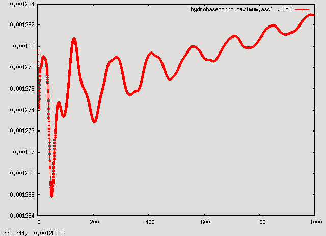
In this case it's interesting to look at the maximum of the density (in the file hydrobase::rho.maximum.asc). Start gnuplot with the command:
gnuplot
and at the gnuplot prompt type:
p 'hydrobase::rho.maximum.asc' u 2:3 w lp
This plots the data in column 3 (rho) as a function of the data in column 2 (time).
As can be seen from the plot, the maximum of the density oscillates with decreasing amplitude around the initial value with a small drift upwards. Even though the initial model is supposed to be in equilibrium, numerical errors means that the numerical model is not exactly in equilibrium and it starts to oscillate. The oscillation energy is slowly dissipated by shocks, decreasing the oscillation amplitude, while the star contracts in response, increasing the maximum density.
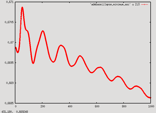
A consistent picture can be seen by plotting the minimum of the lapse:
p 'admbase::lapse.minimum.asc' u 2:3 w lp
The quantity shows the same features as the maximum of the density, except the drift is downwards. The downwards trend stems from the contraction of the star. As the star contracts, the curvature of spacetime increases slightly. In response, the singularity avoiding lapse condition used here decreases the lapse.
As the oscillations and subsequent drift of the density and the lapse are caused by numerical error, increasing the numerical resolution will decrease these effects.
Additional Example Parameter Files
In addition to the TOV star parameter file, we also provide a couple of vacuum parameter files: ks-mclachlan.par and qc0-mclachlan.par. The first (ks-mclachlan.par) evolves a single isolated rotating black hole with the initial data (M=1 and a/M=0.8) specified in Kerr-Schild coordinates. The second (qc0-mclachlan.par) evolves a binary black hole system using the moving puncture technique. The black holes start at a close separation and only complete about one half of an orbit before merging. You can run these additional parameter files using a similar command in the Cactus directory as for the TOV star above:
./simfactory/sim create-submit ks-mclachlan --parfile=par/ks-mclachlan.par --procs=32 --walltime=8:0:0
and
./simfactory/sim create-submit qc0-mclachlan --parfile=par/qc0-mclachlan.par --procs=32 --walltime=8:0:0
Any Problems?
This example should work smoothly on the TeraGrid machines Queen Bee, Ranger, Kraken and Abe. If you have any problems, please send details to users@einsteintoolkit.org.

