Simplified Tutorial for New Users

Here you will find a concise and straightforward guide to downloading, installing, and running the Einstein Toolkit. For a more detailed tutorial, view the Tutorial for New Users.

Prerequisites

You will need a number of packages installed in order to download the Einstein Toolkit components, and if you follow the instructions in this tutorial. On a Debian, Linux-Mint or Fedora-based system, install them as follows:

# Debian (squeeze)
su apt-get install build-essential g++ gfortran libmpich2-dev mercurial git subversion curl gnuplot
# Mint13 (likely Ubuntu oneiric ocelot as well)
sudo apt-get install libmpich2-dev gfortran g++ git mercurial subversion curl gnuplot
# Fedora (incomplete)
yum install git wget

Downloading

A script called GetComponents is used to fetch the components of the Einstein Toolkit. You may download it as follows:

curl -O https://raw.github.com/gridaphobe/CRL/ET_2012_05/GetComponents
chmod a+x GetComponents

GetComponents accepts a thorn list as an argument. To check out the needed components:

./GetComponents --parallel https://svn.einsteintoolkit.org/manifest/branches/ET_2012_05/einsteintoolkit.th

This checks out Cactus, the Einstein Toolkit, and Simulation Factory.

Configuring

You may proceed to configure Simfactory which requires some changes for some OS.

cd Cactus
# for Mint13 (mpich2 needs mpl)
sed '/MPI_LIBS/s/mpich/mpich mpl/' <simfactory/mdb/optionlists/debian.cfg >simfactory/mdb/optionlists/mint.cfg
./simfactory/bin/sim setup --optionlist=mint.cfg
# for Debian
./simfactory/bin/sim setup --optionlist=debian.cfg
# for Fedora
./simfactory/bin/sim setup --optionlist=fedora.cfg

Accept the default values for all options.

Building

Now that you have configured Simfactory, you may build:

./simfactory/bin/sim build --thornlist=manifest/einsteintoolkit.th

This may take a while, as it compiles all the thorns specified in manifest/einsteintoolkit.th.

Running

The example files provided at for the most part too large to run on a single machine. You can try however to run the static_tov example which is smallest and requires about 1.3GB of RAM to run and will run for about 24 hours using a single core. To speed up the run, you can try and reduce the resolution by increasing the parameters "CoordBase::dx", "CoordBase::dy", and "CoordBase::dz" from 8 to 12 whic will reduce runtime to roughly 5 hours and memory consumption to 800MB.

 sed '/CoordBase::d[xyz]/s/8/12/' <par/static_tov.par >par/static_tov_small.par
 ./simfactory/bin/sim submit static_tov --parfile=par/static_tov_small.par --procs=1 --walltime=8:0:0
 ./simfactory/bin/sim show-output --follow static_tov

Look at Results

When the simulation is complete (ie. when "All done" appears in the output), stop simfactory by pressing CTRL-C and move to the output directory. The command should be:

cd ~/simulations/static_tov/output-0000/static_tov

You should see a number of files with the extenstion .asc. These are 0-D (reductions of 3-D grid functions to scalar values) and 1-D ASCII output files that can be plotted with gnuplot.

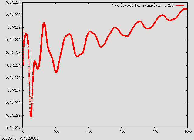
In this case it's interesting to look at the maximum of the density (in the file hydrobase::rho.maximum.asc). Start gnuplot with the command:

gnuplot

and at the gnuplot prompt type:

plot 'hydrobase::rho.maximum.asc' using 2:3 with linespoints

This plots the data in column 3 (rho) as a function of the data in column 2 (time).

As can be seen from the plot, the maximum of the density oscillates with decreasing amplitude around the initial value with a small drift upwards. Even though the initial model is supposed to be in equilibrium, numerical errors means that the numerical model is not exactly in equilibrium and it starts to oscillate. The oscillation energy is slowly dissipated by shocks, decreasing the oscillation amplitude, while the star contracts in response, increasing the maximum density.

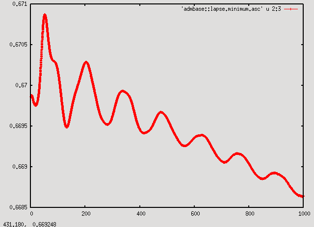
A consistent picture can be seen by plotting the minimum of the lapse:

p 'admbase::lapse.minimum.asc' u 2:3 w lp

The quantity shows the same features as the maximum of the density, except the drift is downwards. The downwards trend stems from the contraction of the star. As the star contracts, the curvature of spacetime increases slightly. In response, the singularity avoiding lapse condition used here decreases the lapse.

As the oscillations and subsequent drift of the density and the lapse are caused by numerical error, increasing the numerical resolution will decrease these effects.